Comparing Attrition with Kaplan and Meier Estimation
We introduced Attrition Analysis in Human Resources Management using the Kaplan and Meier Estimation in a previous post of this blog. In summary, we can say that the Kaplan and Meier Estimation (a non-parametric method) defines a survival function that allows us to calculate the probability (\(S(t)\)) that one employee leaves the organization after a while.
In the previous post, we explained how to calculate the survival function of all employees, understand the results, and represent it. Today, we will see how to calculate the survival function of two (or more) employee groups (e.g., employees from different departments) of the same organization and test whether we could consider if their survival functions are different.
We will use the same data set (ibm_employees_attrition_performance) as the last time, which we can find in the package HRdatsets. This data set contains a sample of 1,472 employees.
library(tidyverse)
devtools::install_github("vicencfernandez/HRdatasets")
library(HRdatasets)
We need two packages to carry out the Attrition Analysis with the Kaplan and Meier Estimation: the survival and the survminer packages.
library(survival)
library(survminer)
After loading them, the following step is to create a survival object with the information of employees. Usually, we only need two variables: the time (years) that each employee has been in the company in the period that we are analyzing (in our case, the variable years), and if finally, the employee left the organization during the period that we are studying (in our case, the variable attrition). But now, we need a third variable to cluster the employees in two or more groups. On this occasion, we have decided to use the variable gender for clustering the employee sample.
# Select the two core variables and the segmentation variable, and transform the variable attrition
employee.clean <- ibm_employees_attrition_performance %>%
  select (Attrition, YearsAtCompany, Gender) %>%
  rename (attrition = Attrition, years = YearsAtCompany, gender = Gender) %>%
  mutate (attrition = if_else(attrition=="Yes", 1, 0))

# Build the survival object with the two core variables
employee.surv <- Surv(time = employee.clean$years, event = employee.clean$attrition)
From the survival object, we will carry out our survival analysis with the function survfit. There are three parameters:
- function - where we need to include the survival object. As we want to analyze our data set depending on the gender, we write
~gender. - data - the data set that we are analyzing
- type - The type of estimation that we want to carry out. In this case, we are going to use the Kaplan and Meier Estimation.
employee.km <- survfit(employee.surv ~ gender, data = employee.clean, type = "kaplan-meier")

# Some results
print(employee.km)
## Call: survfit(formula = employee.surv ~ gender, data = employee.clean,
## type = "kaplan-meier")
##
## n events median 0.95LCL 0.95UCL
## gender=Female 590 89 32 32 NA
## gender=Male 882 150 NA 31 NA# More results
summary(employee.km)## Call: survfit(formula = employee.surv ~ gender, data = employee.clean,
## type = "kaplan-meier")
##
## gender=Female
## time n.risk n.event survival std.err lower 95% CI upper 95% CI
## 0 590 4 0.993 0.00338 0.9866 1.000
## 1 575 21 0.957 0.00842 0.9406 0.974
## 2 511 10 0.938 0.01013 0.9186 0.958
## 3 467 7 0.924 0.01129 0.9023 0.947
## 4 411 5 0.913 0.01222 0.8893 0.937
## 5 376 9 0.891 0.01393 0.8642 0.919
## 6 289 3 0.882 0.01477 0.8533 0.911
## 7 260 5 0.865 0.01632 0.8335 0.897
## 8 224 4 0.849 0.01776 0.8153 0.885
## 9 187 4 0.831 0.01957 0.7938 0.870
## 10 151 6 0.798 0.02297 0.7544 0.845
## 11 115 1 0.791 0.02380 0.7460 0.839
## 13 94 1 0.783 0.02499 0.7354 0.833
## 15 74 1 0.772 0.02680 0.7215 0.827
## 17 58 1 0.759 0.02946 0.7034 0.819
## 22 20 1 0.721 0.04638 0.6356 0.818
## 24 13 1 0.666 0.06835 0.5442 0.814
## 32 5 2 0.399 0.15147 0.1899 0.840
## 33 3 2 0.133 0.11984 0.0228 0.777
## 40 1 1 0.000 NaN NA NA
##
## gender=Male
## time n.risk n.event survival std.err lower 95% CI upper 95% CI
## 0 882 12 0.986 0.00390 0.979 0.994
## 1 853 38 0.942 0.00790 0.927 0.958
## 2 746 17 0.921 0.00928 0.903 0.939
## 3 663 13 0.903 0.01036 0.883 0.923
## 4 591 14 0.882 0.01159 0.859 0.905
## 5 516 12 0.861 0.01274 0.836 0.886
## 6 407 6 0.848 0.01356 0.822 0.875
## 7 360 6 0.834 0.01452 0.806 0.863
## 8 306 5 0.821 0.01551 0.791 0.852
## 9 263 4 0.808 0.01648 0.776 0.841
## 10 217 12 0.763 0.01999 0.725 0.804
## 11 133 1 0.758 0.02065 0.718 0.799
## 13 108 1 0.751 0.02161 0.709 0.794
## 14 94 2 0.735 0.02392 0.689 0.783
## 16 76 1 0.725 0.02549 0.677 0.777
## 18 66 1 0.714 0.02737 0.662 0.770
## 19 60 1 0.702 0.02938 0.647 0.762
## 20 55 1 0.689 0.03150 0.630 0.754
## 21 42 1 0.673 0.03476 0.608 0.745
## 23 26 1 0.647 0.04197 0.570 0.735
## 31 13 1 0.597 0.06154 0.488 0.731With these results, we can analyze the survival probability for each time in each gender. For instance, in the case of females, there is a 79.1% (survival) of the probability of surviving (to keep working in the organization) during 11 months (t). There was 1 (n.event) female who left the organization in the 11th month in our data set, and there were 115 females (n.risk) with probabilities to leave the organization in the 11th month. On the other hand, for males, there is a 75.8% (survival) of the probability of surviving during 11 months (t). There was 1 (n.event) male who left the organization in the 11th month in our data set, and there were 133 females (n.risk) with probabilities to leave the organization in the 11th month.
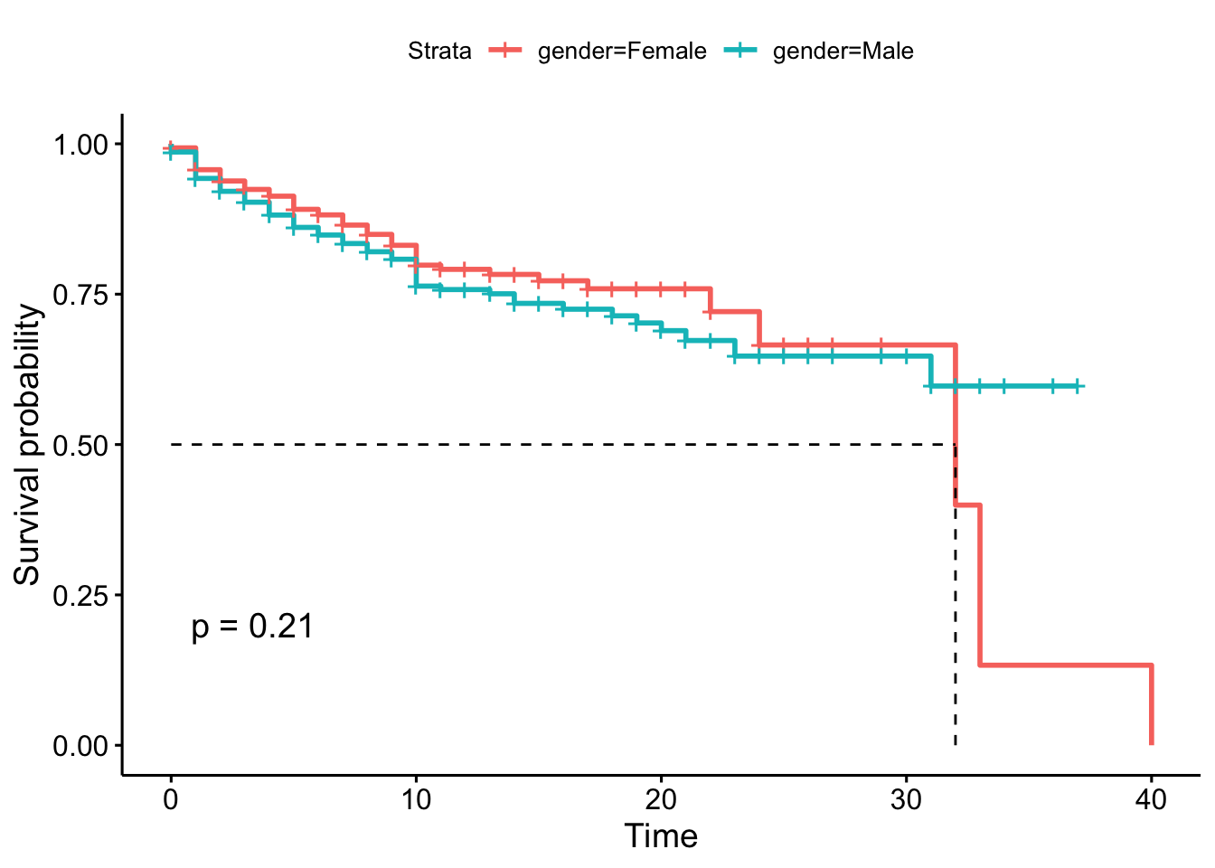
It’s also widespread to show the survival probabilities using Survival Curves. Let’s see the previous example, and if we can confirm that the survival functions are different depending on the gender.
ggsurvplot(employee.km, surv.median.line = "hv")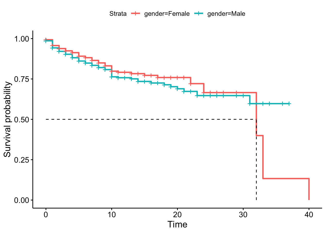
In some cases, it’s effortless to test if the survival curves are different. But in this specific case, it isn’t easy to decide if these two survival functions are significantly different based on the survival curves. In some parts, they are very similar, but not in others. One option to take this decision is to carry out a log-rank test (the log-rank statistic is approximately distributed as a chi-square test statistic).
# Long-Rank Test
survdiff(employee.surv ~ gender, data = employee.clean, rho = 0)
## Call:
## survdiff(formula = employee.surv ~ gender, data = employee.clean,
## rho = 0)
##
## N Observed Expected (O-E)^2/E (O-E)^2/V
## gender=Female 590 89 98.3 0.884 1.55
## gender=Male 882 150 140.7 0.618 1.55
##
## Chisq= 1.6 on 1 degrees of freedom, p= 0.2As the p-value is greater than 0.05 (the typical threshold), we cannot reject the hypothesis that the survival curves (probabilities) are the same in both populations over time. So, we need to consider that the attrition for females and males are the same. We also can get the p-value of the log-rank test adding the parameter pval = TRUE in the visual representation.
ggsurvplot(employee.km, pval = TRUE, surv.median.line = "hv")