Attrition Analysis with Kaplan and Meier Estimation
Attrition Analysis is one of the most common analyses that companies carry out. The loss of talented employees and finding and training new ones could take a long time, lose a competitive advantage, and generate elevated costs.
Attrition Analysis belongs to the Survival Analysis category, and there are three basic approaches to analyze it.
- Parametric methods
- Semi-parametric methods
- Non-parametric methods
Today, we will see the most popular non-parametric method for the attrition analysis: The Kaplan and Meier Estimation. One of the most interesting characteristics of the non-parametric methods is that the sample doesn’t have to satisfy any distribution. However, before starting with an example, we need to introduce some basic concepts.
The Kaplan and Meier Estimation defines a survival function (\(S(t)\)) that depends on time and tells us the probability that one employee will keep working in the company at a specific time. At the beginning of the process, the probability of surviving is one (\(S(t=0)=1\)). When the time tends to infinity, the probability of surviving is zero (\(S(t \rightarrow \infty)=0\)). Finally, we need to take into account the survival function cannot increase with time.
Now, we can start with an example. Firstly, we need to load the data set ibm_employees_attrition_performance to find in the package HRdatsets. This data set contains a sample with 1,472 employees.
library(tidyverse)

devtools::install_github("vicencfernandez/HRdatasets")
library(HRdatasets)
ibm_employees_attrition_performance
## # A tibble: 1,472 x 35
## Age Attrition BusinessTravel DailyRate Department DistanceFromHome
## <int> <chr> <chr> <int> <chr> <int>
## 1 41 Yes Travel_Rarely 1102 Sales 1
## 2 49 No Travel_Frequent… 279 Research & Devel… 8
## 3 37 Yes Travel_Rarely 1373 Research & Devel… 2
## 4 33 No Travel_Frequent… 1392 Research & Devel… 3
## 5 27 No Travel_Rarely 591 Research & Devel… 2
## 6 32 No Travel_Frequent… 1005 Research & Devel… 2
## 7 59 No Travel_Rarely 1324 Research & Devel… 3
## 8 30 No Travel_Rarely 1358 Research & Devel… 24
## 9 38 No Travel_Frequent… 216 Research & Devel… 23
## 10 36 No Travel_Rarely 1299 Research & Devel… 27
## # … with 1,462 more rows, and 29 more variables: Education <int>,
## # EducationField <chr>, EmployeeCount <int>, EmployeeNumber <int>,
## # EnvironmentSatisfaction <int>, Gender <chr>, HourlyRate <int>,
## # JobInvolvement <int>, JobLevel <int>, JobRole <chr>, JobSatisfaction <int>,
## # MaritalStatus <chr>, MonthlyIncome <int>, MonthlyRate <int>,
## # NumCompaniesWorked <int>, Over18 <chr>, OverTime <chr>,
## # PercentSalaryHike <int>, PerformanceRating <int>,
## # RelationshipSatisfaction <int>, StandardHours <int>,
## # StockOptionLevel <int>, TotalWorkingYears <int>,
## # TrainingTimesLastYear <int>, WorkLifeBalance <int>, YearsAtCompany <int>,
## # YearsInCurrentRole <int>, YearsSinceLastPromotion <int>,
## # YearsWithCurrManager <int>We need two ’ packages’ to carry out the Attrition Analysis with the Kaplan and Meier Estimation. The survival package contains the core survival analysis routines, including the definition of Surv objects, Kaplan-Meier and Aalen-Johansen (multi-state) curves, Cox models, and parametric accelerated failure time models. The survminer package contains functions for drawing effortlessly beautiful and ‘ready-to-publish’ survival curves with the ‘number at risk’ table and ‘censoring count plot’.
library(survival)
library(survminer)
Now, we need to build a Survival object with the information of employees. We only need two variables: the time (years) that each employee has been in the company in the period that we are analyzing (in our case, the variable years), and if finally, the employee left the organization during the period that we are studying (in our case, the variable attrition).
# Select the two core variables, and transform the variable attrition
employee.clean <- ibm_employees_attrition_performance %>%
  select (Attrition, YearsAtCompany) %>%
  rename (attrition = Attrition, years = YearsAtCompany) %>%
  mutate (attrition = if_else(attrition=="Yes", 1, 0))

employee.surv <- Surv(time = employee.clean$years, event = employee.clean$attrition)
head (employee.surv, 30)
## [1] 6 10+ 0 8+ 2+ 7+ 1+ 1+ 9+ 7+ 5+ 9+ 5+ 2+ 4 10+ 6+ 1+ 25+
## [20] 3+ 4+ 5 12+ 0+ 4 14+ 10 9+ 22+ 2+The object employee.surv shows the times and the attrition with the symbol + of all the employees. With this object, we calculate the survival analysis with the function survfit. There are three parameters:
- function - where we need to include the survival object. As we don’t want to analyze our data set taking into account other variables, we write 1
- data - the data set that we are analyzing
- type - The type of estimation that we want to carry out. In this case, we are going to use the Kaplan and Meier Estimation.
employee.km <- survfit(employee.surv ~ 1, data = employee.clean, type = "kaplan-meier")

# Some results
print(employee.km)
## Call: survfit(formula = employee.surv ~ 1, data = employee.clean, type = "kaplan-meier")
##
## n events median 0.95LCL 0.95UCL
## 1472 239 33 32 NA# More results
summary(employee.km)## Call: survfit(formula = employee.surv ~ 1, data = employee.clean, type = "kaplan-meier")
##
## time n.risk n.event survival std.err lower 95% CI upper 95% CI
## 0 1472 16 0.989 0.00270 0.984 0.994
## 1 1428 59 0.948 0.00582 0.937 0.960
## 2 1257 27 0.928 0.00689 0.914 0.941
## 3 1130 20 0.911 0.00768 0.897 0.927
## 4 1002 19 0.894 0.00850 0.878 0.911
## 5 892 21 0.873 0.00946 0.855 0.892
## 6 696 9 0.862 0.01006 0.842 0.882
## 7 620 11 0.847 0.01089 0.825 0.868
## 8 530 9 0.832 0.01171 0.810 0.855
## 9 450 8 0.817 0.01261 0.793 0.842
## 10 368 18 0.777 0.01511 0.748 0.808
## 11 248 2 0.771 0.01563 0.741 0.802
## 13 202 2 0.764 0.01638 0.732 0.796
## 14 178 2 0.755 0.01728 0.722 0.790
## 15 160 1 0.750 0.01781 0.716 0.786
## 16 140 1 0.745 0.01847 0.710 0.782
## 17 128 1 0.739 0.01922 0.702 0.778
## 18 119 1 0.733 0.02003 0.695 0.773
## 19 106 1 0.726 0.02100 0.686 0.768
## 20 95 1 0.718 0.02213 0.676 0.763
## 21 68 1 0.708 0.02419 0.662 0.757
## 22 54 1 0.695 0.02706 0.644 0.750
## 23 39 1 0.677 0.03169 0.617 0.742
## 24 37 1 0.658 0.03573 0.592 0.732
## 31 18 1 0.622 0.04902 0.533 0.726
## 32 15 2 0.539 0.06917 0.419 0.693
## 33 11 2 0.441 0.08445 0.303 0.642
## 40 1 1 0.000 NaN NA NAWith these results, we can analyze the survival probability for each time. For instance, there is a 77.0% (survival) of probabilities of surviving (to keep working in the organization) during 11 months (t). There are 2 (n.event) employees who left the organization in the 11th month in our data set, and there were 246 (n.risk) with probabilities to leave the organization in the 11th month.
It’s also widespread to show the survival probabilities using Survival Curves. Let’s see the example.
ggsurvplot(employee.km, surv.median.line = "hv")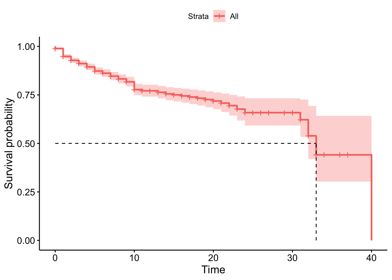
As we can see in the previous plot, there is a 50% of probabilities to survive (keep working in the same company) during 32 years.